Research Results:RQ3_2021
Simulation of infection spread and control
-
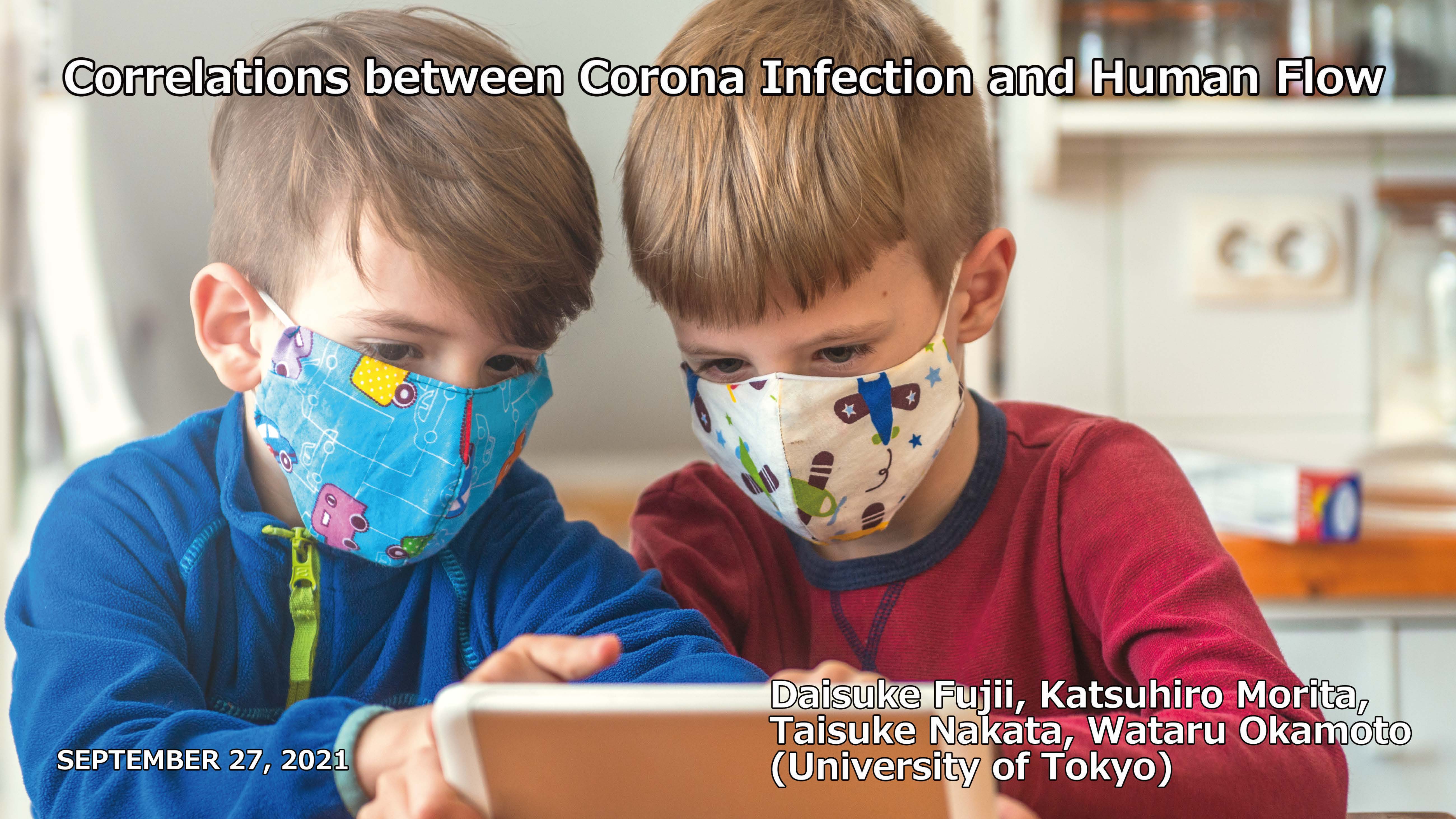
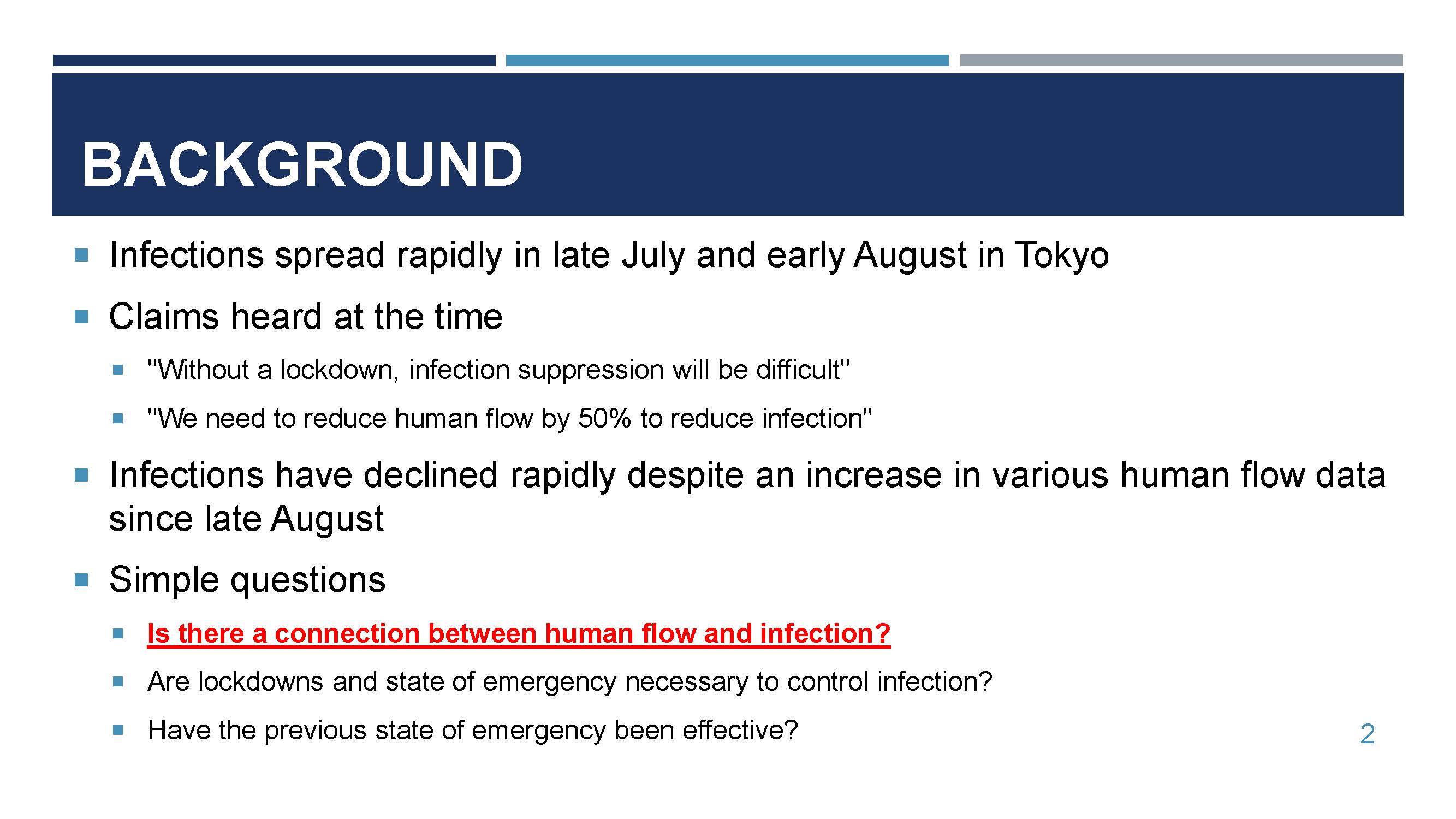
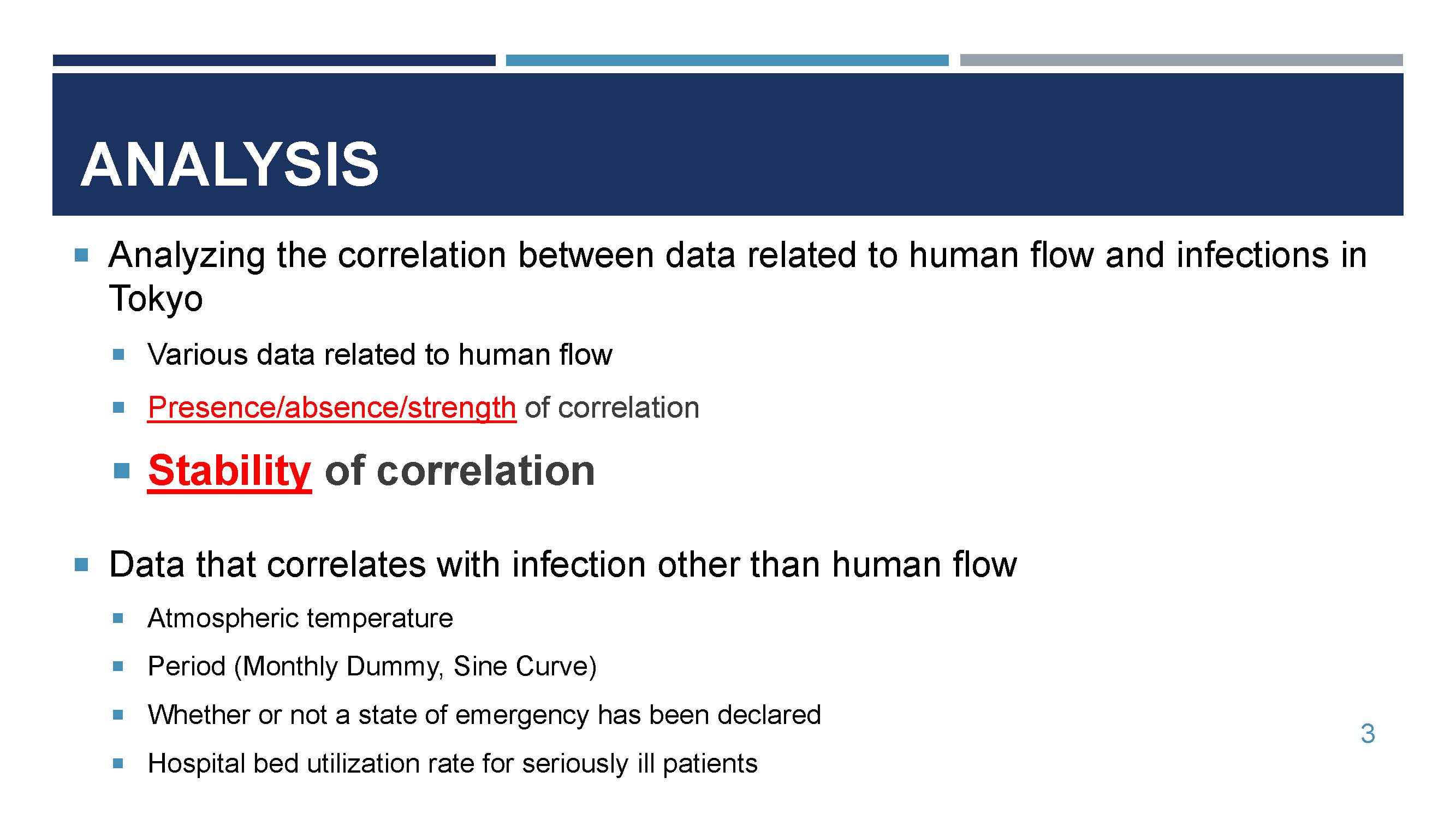
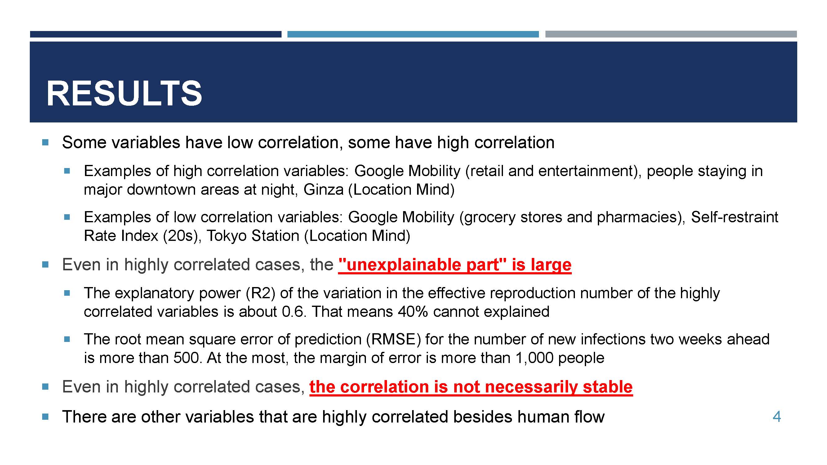
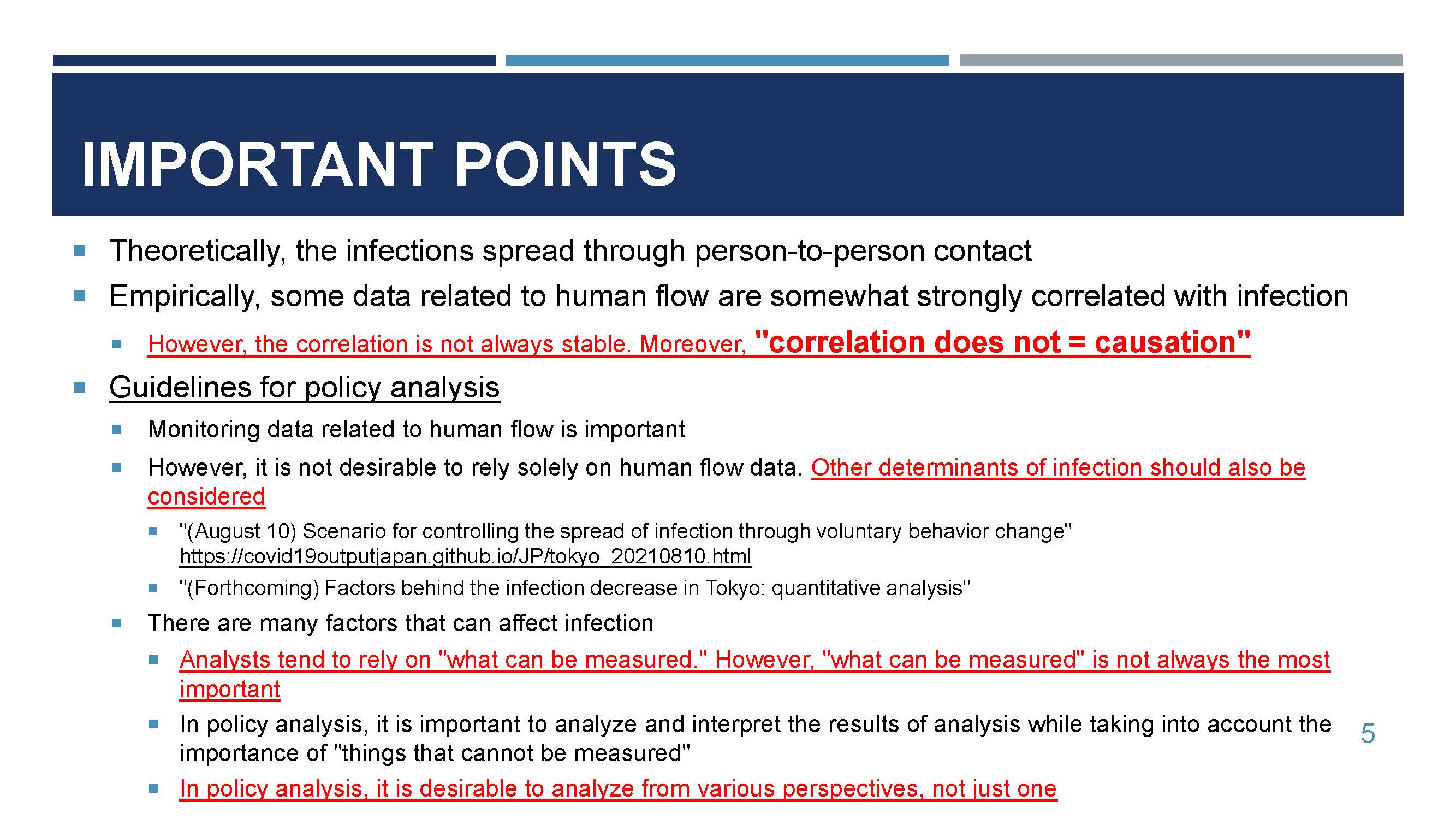
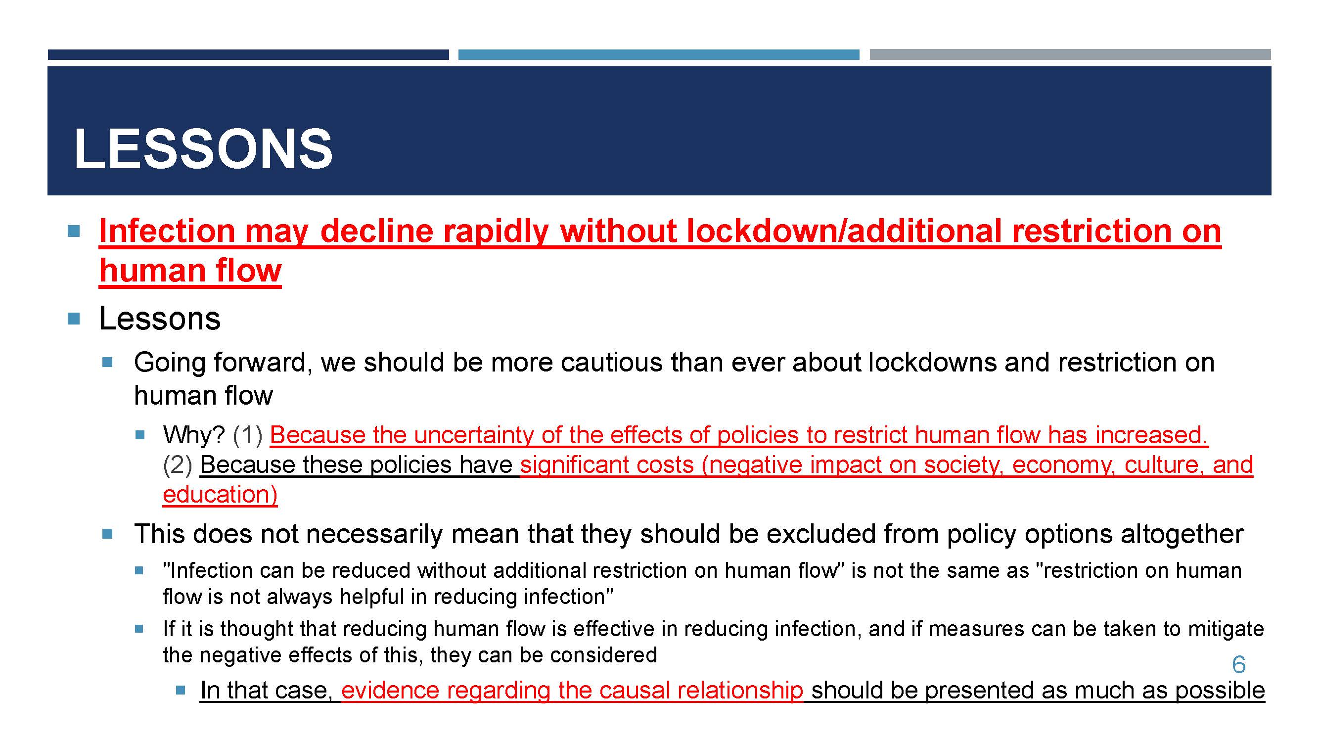
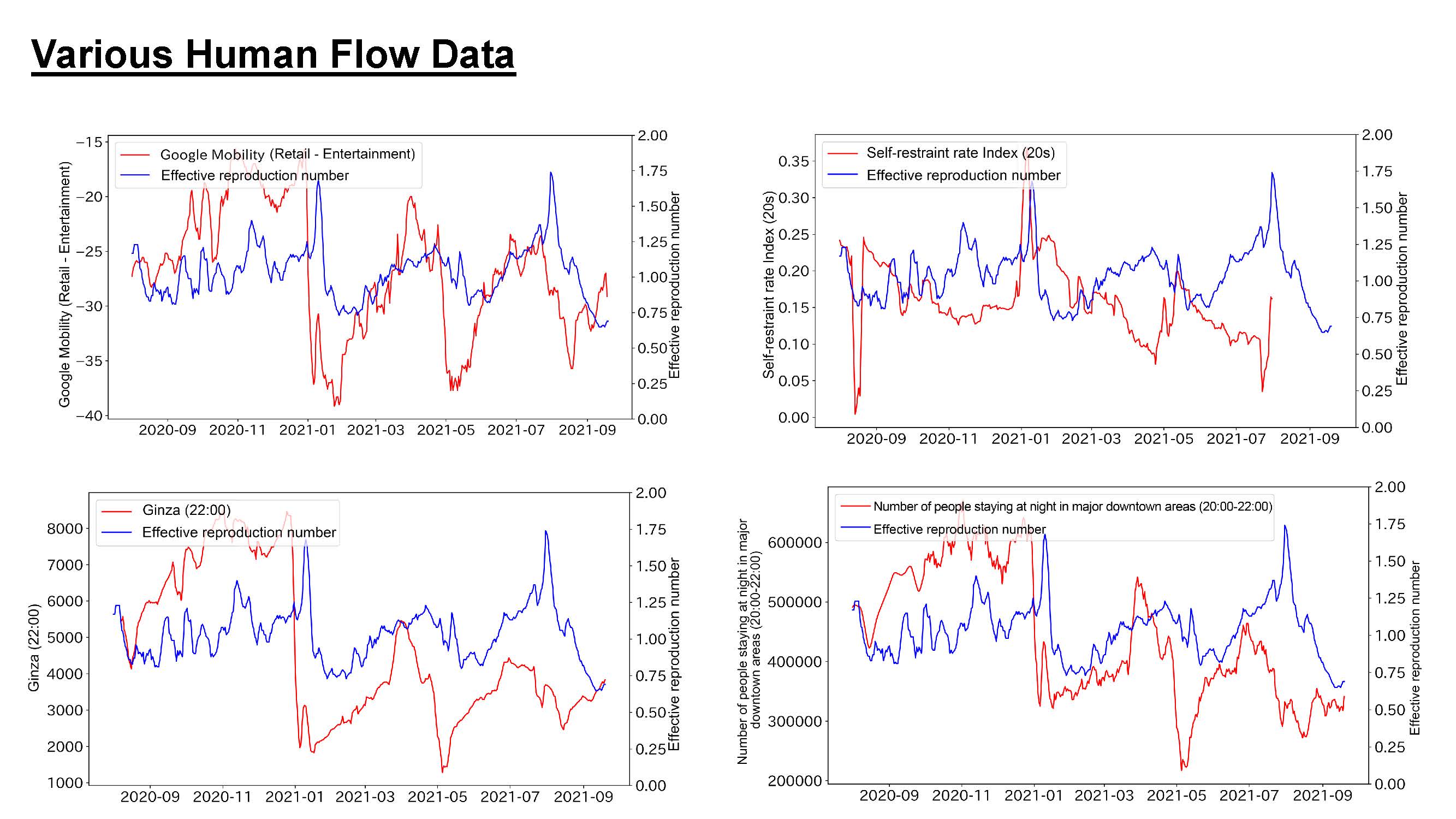
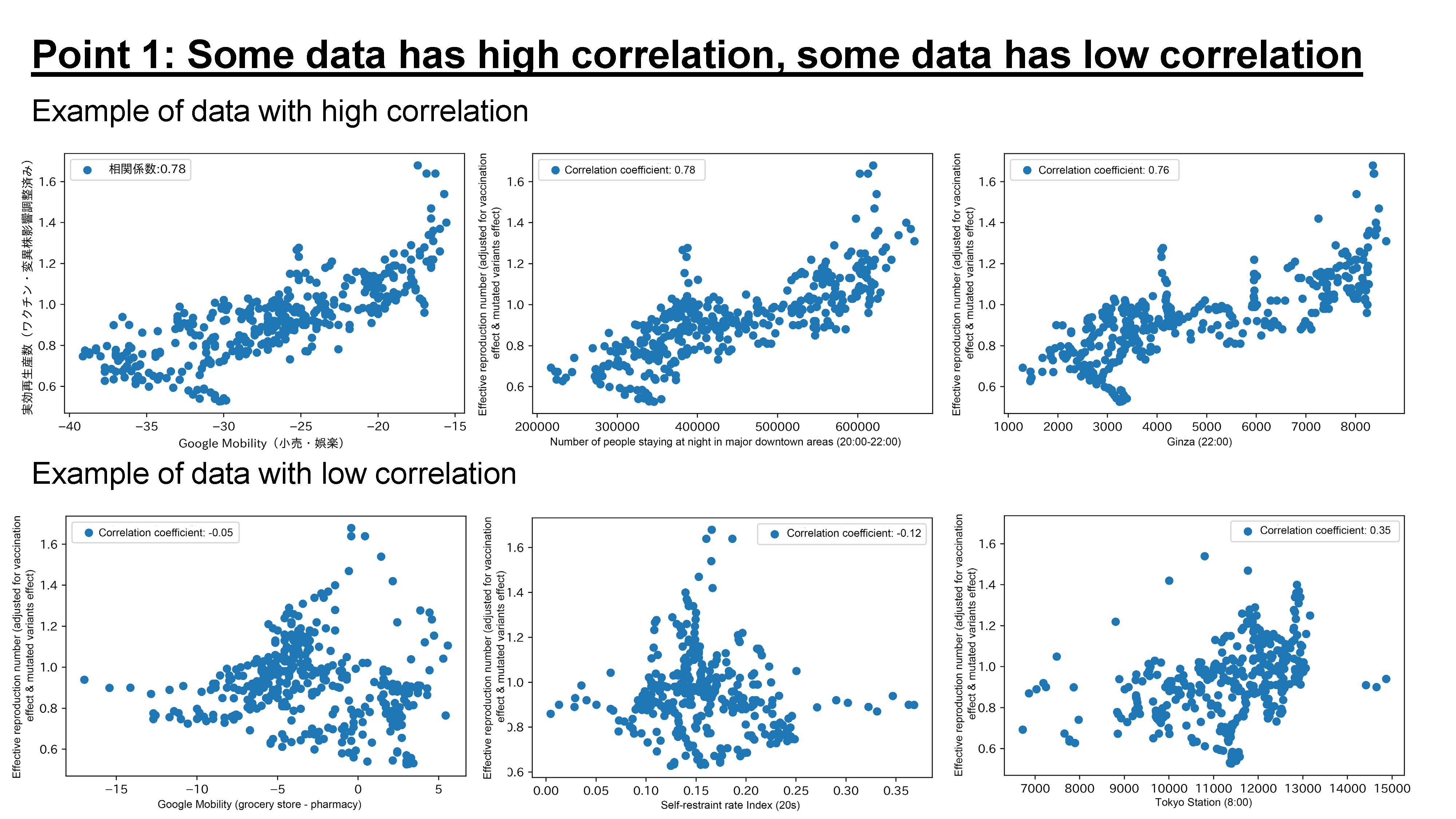
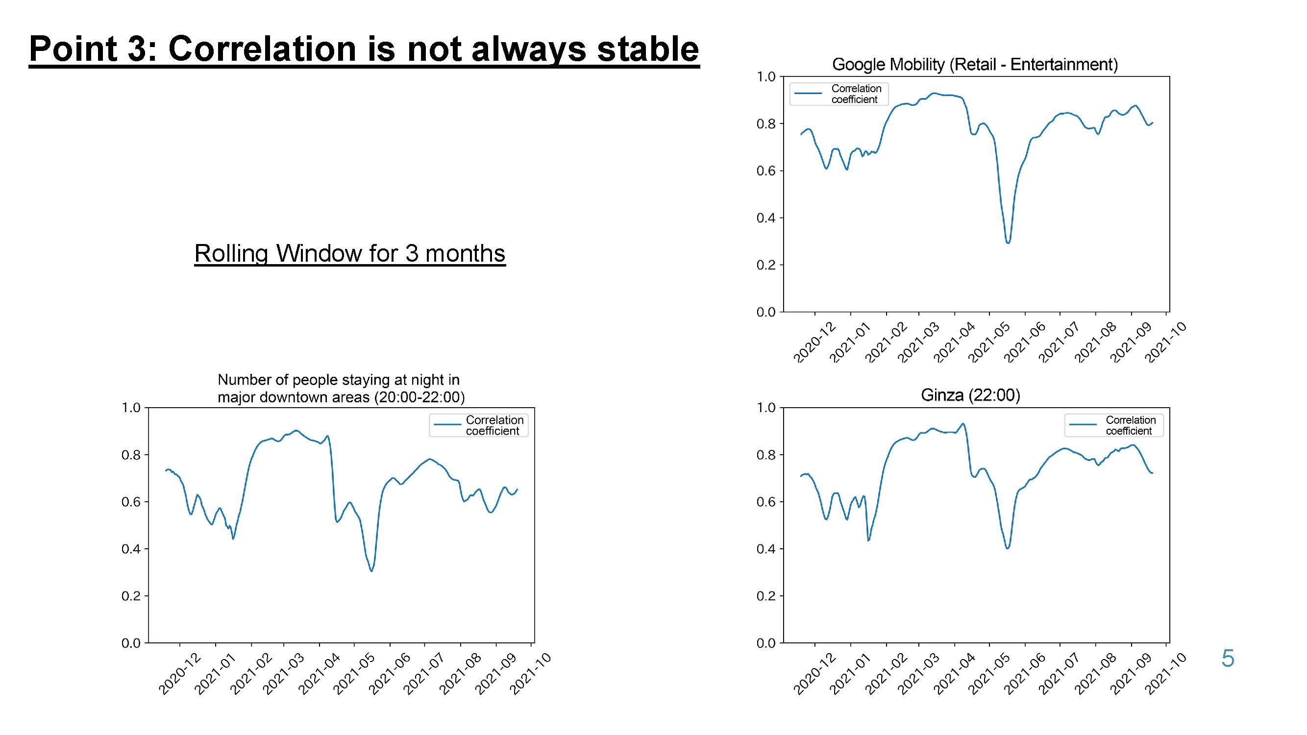
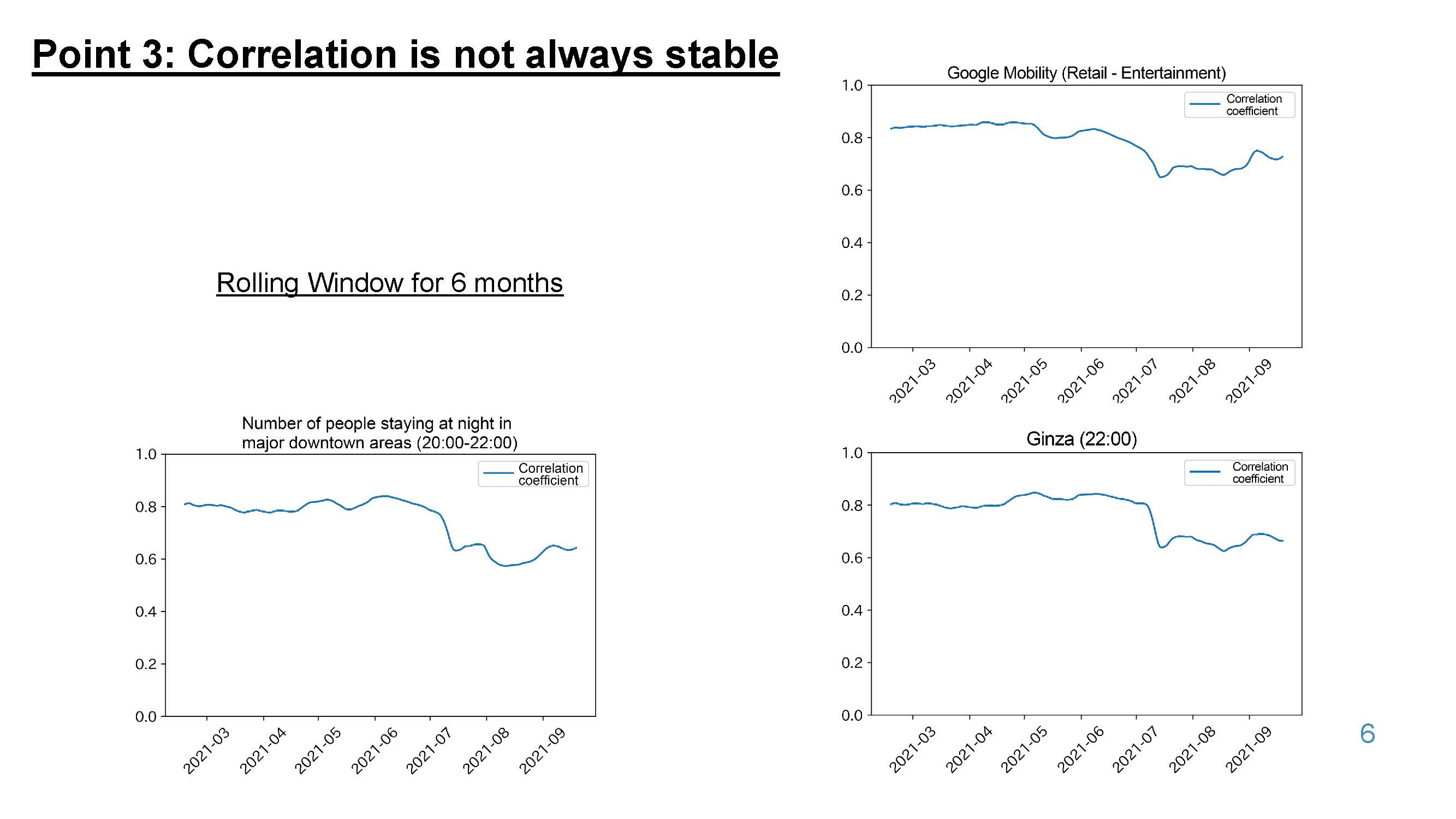
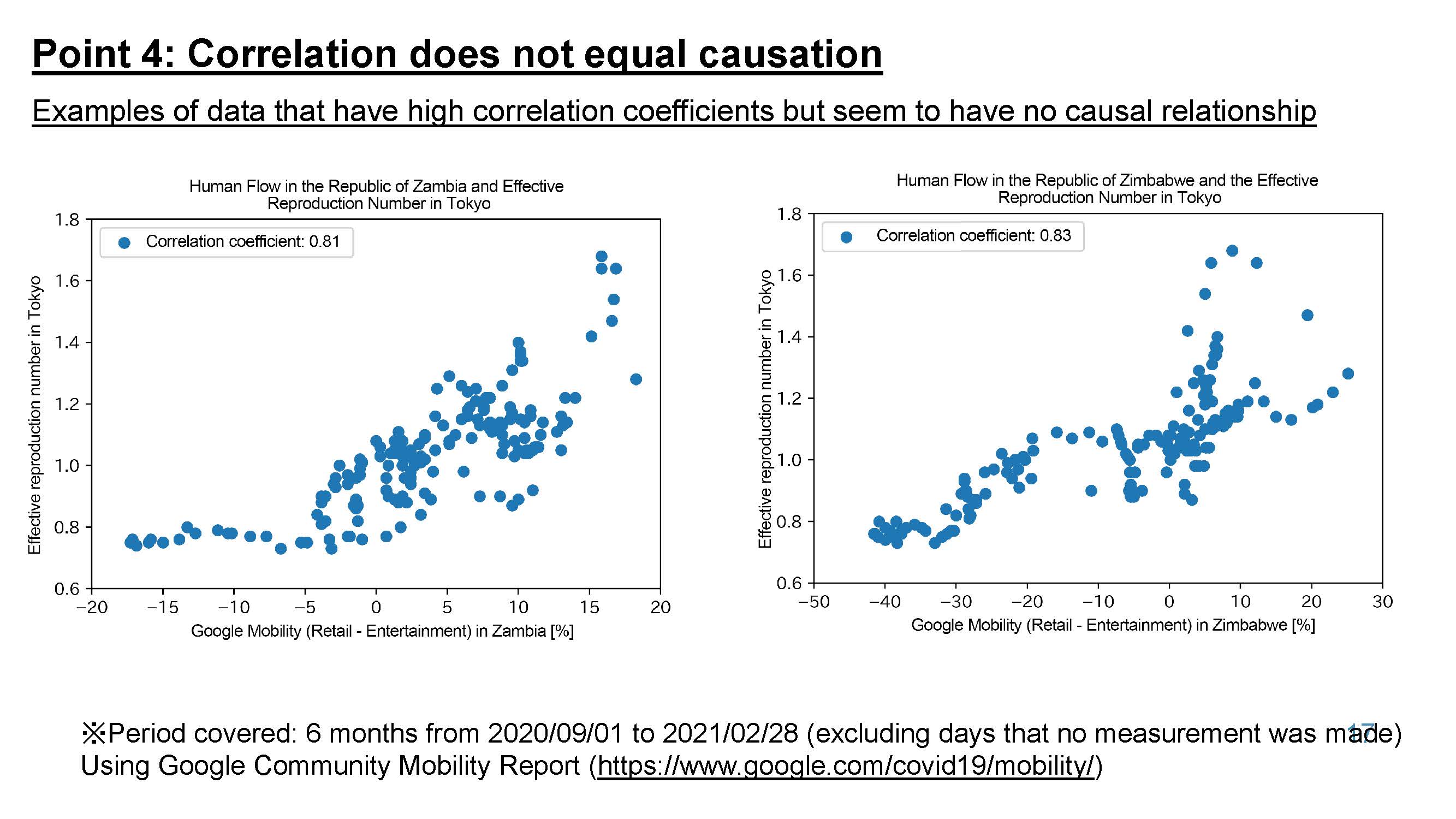
Correlations between Corona Infection and Human Flow
2021.09.29
Researcher
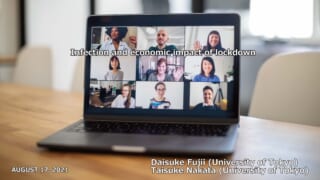
Taisuke Nakata
-
-
Related reports

Researcher
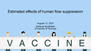
Setsuya Kurahashi
Researcher
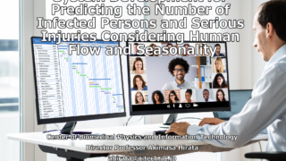
Akimasa Hirata
Researcher
Taisuke Nakata
Organization
The University of Tokyo (School of Engineering)
Researcher
Yukio Ohsawa
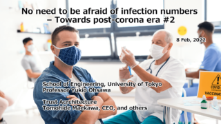
No need to be afraid of infection numbers – In the case of the low severity rate scenario #4
2022.03.08
Organization
The University of Tokyo (School of Engineering)
Researcher
Yukio Ohsawa

Researcher
Akimasa Hirata
Researcher
Taisuke Nakata
Organization
The Tokyo Foundation for Policy Research
Researcher
Asako Chiba
Divorce rates during COVID-19
2022.03.08
Organization
The Tokyo Foundation for Policy Research
Researcher
Asako Chiba

Researcher
Akimasa Hirata
Organization
The Tokyo Foundation for Policy Research
Researcher
Asako Chiba
Marriage and birth rates during COVID-19
2022.03.01
Organization
The Tokyo Foundation for Policy Research
Researcher
Asako Chiba

Researcher
Akimasa Hirata


Organization
The University of Tokyo (School of Engineering)
Researcher
Yukio Ohsawa
Researcher
Setsuya Kurahashi
Organization
The Tokyo Foundation for Policy Research
Researcher
Asako Chiba


Researcher
Akimasa Hirata

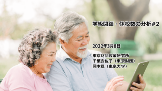
Estimates of the number of daycare closures
2022.02.15
Organization
The Tokyo Foundation for Policy Research
Researcher
Asako Chiba
Researcher
Akimasa Hirata
Organization
The University of Tokyo (School of Engineering)
Researcher
Yukio Ohsawa
Researcher
Setsuya Kurahashi
Researcher
Taisuke Nakata
Researcher
Taisuke Nakata
Birth rates during COVID-19
2022.02.08
Organization
The Tokyo Foundation for Policy Research
Researcher
Asako Chiba
Marriage rates during COVID-19
2022.02.08
Organization
The Tokyo Foundation for Policy Research
Researcher
Asako Chiba

Researcher
Tatsuo Unemi

Researcher
Akimasa Hirata
Researcher
Taisuke Nakata
Researcher
Tatsuo Unemi
Researcher
Akimasa Hirata
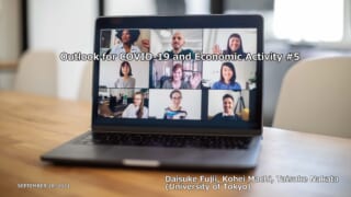
Outlook for COVID-19 and Economic Activity – Impact of stricter hospitalization standards #9
2022.01.25
Researcher
Taisuke Nakata
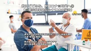
No need to be afraid of infection numbers – Towards post-corona era (low severity scenario)
2022.01.25
Researcher
Yukio Ohsawa
Researcher
Setsuya Kurahashi
Researcher
Setsuya Kurahashi

Researcher
Tatsuo Unemi
Researcher
Setsuya Kurahashi
Researcher
Akimasa Hirata
Organization
The Tokyo Foundation for Policy Research
Researcher
Asako Chiba
Researcher
Taisuke Nakata
Researcher
Taisuke Nakata
Researcher
Setsuya Kurahashi
Organization
The University of Tokyo (School of Engineering)
Researcher
Yukio Ohsawa
Researcher
Taisuke Nakata
Researcher
Akimasa Hirata
Researcher
Akimasa Hirata
Organization
The University of Tokyo (School of Engineering)
Researcher
Yukio Ohsawa
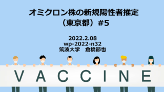
Projection of the number of new positive persons assuming the prevalence of Omicron variant
2021.12.21
Researcher
Akimasa Hirata

Researcher
Tatsuo Unemi
Organization
The Tokyo Foundation for Policy Research
Researcher
Asako Chiba
Researcher
Setsuya Kurahashi
Researcher
Taisuke Nakata

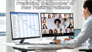
Projection of the number of new positive persons assuming the prevalence of Omicron variant
2021.12.14
Researcher
Akimasa Hirata
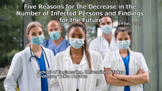
Five Reasons for the Decrease in the Number of Infected Persons and Findings for the Future
2021.12.14
Organization
The University of Tokyo (School of Engineering)
Researcher
Yukio Ohsawa
Researcher
Akimasa Hirata
Researcher
Akimasa Hirata

Researcher
Tatsuo Unemi
Researcher
Akimasa Hirata
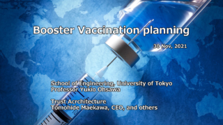
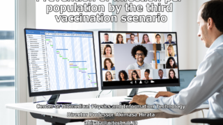
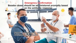
Booster Vaccination planning
2021.11.30
Organization
The University of Tokyo (School of Engineering)
Researcher
Yukio Ohsawa
Organization
The Tokyo Foundation for Policy Research
Researcher
Asako Chiba
Researcher
Setsuya Kurahashi
Researcher
Akimasa Hirata
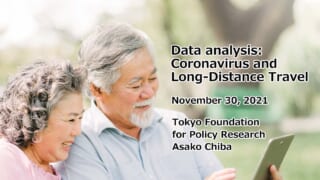
Impact of active domestic travels
2021.11.16
Organization
The Tokyo Foundation for Policy Research
Researcher
Asako Chiba
Researcher
Setsuya Kurahashi
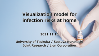
Revised plan of the new Shimoda Model
2021.11.16
Organization
The University of Tokyo (School of Engineering)
Researcher
Yukio Ohsawa
Researcher
Akimasa Hirata
Organization
The University of Tokyo (School of Engineering)
Researcher
Yukio Ohsawa
Researcher
Taisuke Nakata
Wave Flow in KeyGraph: waves are not over
2021.10.26
Organization
The University of Tokyo (School of Engineering)
Researcher
Yukio Ohsawa
Researcher
Taisuke Nakata
Researcher
Akimasa Hirata

Researcher
Akimasa Hirata
Researcher
Taisuke Nakata
Researcher
Setsuya Kurahashi
Strategy Cocktail
2021.10.05
Organization
The University of Tokyo (School of Engineering)
Researcher
Yukio Ohsawa
Effect of Antibody Cocktail
2021.10.05
Organization
The Tokyo Foundation for Policy Research
Researcher
Asako Chiba

Researcher
Akimasa Hirata

Researcher
Akimasa Hirata
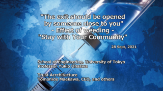
“The exit should be opened by someone close to you” – Effect of weeding – “Stay with Your Community”
2021.09.29
Organization
The University of Tokyo (School of Engineering)
Researcher
Yukio Ohsawa

Researcher
Taisuke Nakata
Researcher
Taisuke Nakata

Researcher
Akimasa Hirata
Organization
Mitsubishi research Institute, Inc.
Organization
The University of Tokyo (School of Engineering)
Researcher
Yukio Ohsawa
Organization
The Tokyo Foundation for Policy Research
Researcher
Asako Chiba
Researcher
Taisuke Nakata
Researcher
Akimasa Hirata
Organization
The University of Tokyo (School of Engineering)
Researcher
Yukio Ohsawa
Researcher
Setsuya Kurahashi
Organization
The Tokyo Foundation for Policy Research
Researcher
Asako Chiba

Researcher
Tatsuo Unemi
Researcher
Tatsuo Unemi

Researcher
Akimasa Hirata
Researcher
Taisuke Nakata
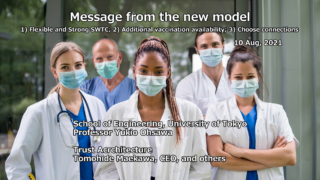
Message from the new model
2021.09.07
Organization
The University of Tokyo (School of Engineering)
Researcher
Yukio Ohsawa
Researcher
Setsuya Kurahashi

Researcher
Akimasa Hirata
Researcher
Taisuke Nakata
Researcher
Setsuya Kurahashi
Organization
Mitsubishi research Institute, Inc.
Organization
The Tokyo Foundation for Policy Research
Researcher
Asako Chiba
Progress on MultiLayer-MultiAgent model
2021.08.24
Organization
The University of Tokyo (School of Engineering)
Researcher
Yukio Ohsawa
Researcher
Taisuke Nakata

Researcher
Taisuke Nakata

Organization
The University of Tokyo (School of Engineering)
Researcher
Yukio Ohsawa
Organization
Mitsubishi research Institute, Inc.

Researcher
Tatsuo Unemi
Researcher
Akimasa Hirata
Researcher
Taisuke Nakata
Researcher
Tatsuo Unemi
Researcher
Taisuke Nakata
Organization
The University of Tokyo (School of Engineering)
Researcher
Yukio Ohsawa
Researcher
Taisuke Nakata

Researcher
Taisuke Nakata
Researcher
Setsuya Kurahashi
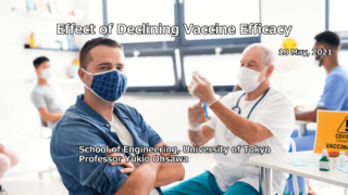
Effect of declining vaccine efficacy
2021.08.03
Organization
The University of Tokyo (School of Engineering)
Researcher
Yukio Ohsawa
Researcher
Tatsuo Unemi

Organization
The University of Tokyo (School of Engineering)
Researcher
Yukio Ohsawa

Researcher
Taisuke Nakata
Researcher
Setsuya Kurahashi
Researcher
Tatsuo Unemi
Organization
The University of Tokyo (School of Engineering)
Researcher
Yukio Ohsawa
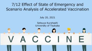
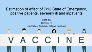
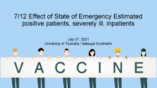
Effectiveness of July 12th Emergency Declaration and Accelerated Vaccination Scenario Analysis
2021.07.20
Researcher
Setsuya Kurahashi


Researcher
Setsuya Kurahashi

Organization
The University of Tokyo (School of Engineering)
Researcher
Yukio Ohsawa
Organization
Mitsubishi research Institute, Inc.
Researcher
Tatsuo Unemi
Organization
Mitsubishi research Institute, Inc.
Researcher
Mitsubishi research Institute, Inc
Researcher
Setsuya Kurahashi
Organization
The University of Tokyo (School of Engineering)
Researcher
Yukio Ohsawa
Organization
The University of Tokyo (School of Engineering)
Researcher
Yukio Ohsawa
Researcher
Setsuya Kurahashi
Organization
Mitsubishi research Institute, Inc.
Researcher
Mitsubishi research Institute, Inc

Researcher
Tatsuo Unemi

Organization
The University of Tokyo (School of Engineering)
Researcher
Yukio Ohsawa
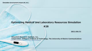
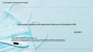
Simulation of Medical and Laboratory Resource Optimization Vaccination Effectiveness Study #4
2021.03.30
Organization
Mitsubishi research Institute, Inc.
Researcher
Mitsubishi research Institute, Inc

Researcher
Tatumi Yamada
Researcher
Setsuya Kurahashi
Researcher
Setsuya Kurahashi
Organization
The University of Tokyo (School of Engineering)
Researcher
Yukio Ohsawa

Simulation of Medical and Laboratory Resource Optimization Vaccination Effectiveness Study #3
2021.03.23
Organization
Mitsubishi research Institute, Inc.
Researcher
Mitsubishi research Institute, Inc
Researcher
Tatsuo Unemi
Organization
Mitsubishi research Institute, Inc.
Researcher
Mitsubishi research Institute, Inc

Researcher
Tatsuo Unemi
Researcher
Setsuya Kurahashi

Simulation of Medical and Laboratory Resource Optimization Vaccination Effectiveness Study #2
2021.03.11
Organization
Mitsubishi research Institute, Inc.
Researcher
Mitsubishi research Institute, Inc
Organization
Mitsubishi research Institute, Inc.
Researcher
Mitsubishi research Institute, Inc
Researcher
Tatsuo Unemi

Organization
Mitsubishi research Institute, Inc.
Researcher
Mitsubishi research Institute, Inc